


Should We Expect Inflation or Deflation?
Money balloon being popped! Image Credit: CanStockPhoto.com/jgroup
Among the most confusing questions of the last decade is whether we are currently in an inflationary economic environment, or not. After all, has not the Federal Reserve been creating money like mad, especially with Quantitative Easing (QE)? Over the years between November 2008 and October 2014, the Federal Reserve bought approximately $4.5 trillion worth of long-term assets under QE – mortgage backed securities and long-term Treasuries. The chart below was produced by the Wall Street Journal at about the same time QE was ended,

This $4.5 trillion in Federal Reserve assets is approximately 25% of the current GDP of about $17.3 trillion! Seeing this amount of new money being created, a great many people expected that run-away inflation would surely follow. For a very long time I was among those expecting inflation just around the corner. Yet horrendous inflation never appeared. Why?
A very big part of this problem’s solution consists of understanding how the QE money fitted in with the all the monetary aggregates: the monetary base, M0, M1, M2, and M3. The other big piece of the puzzle was that only about 20% of the QE money leaked into the economy. The other 80% was frozen in Federal Reserve excess reserves.
First, consider where the QE money belongs in the hierarchy of monetary aggregates. The monetary aggregates M0 through M3 are defined in decreasing states of liquidity. (Note that M0 is not considered a monetary aggregate by the Federal Reserve,)
- M0: Notes and coins in circulation outside Federal Reserve Banks and vaults of depository institutions, in other words, currency.
- M1: M0 plus traveler’s checks of non-bank issuers, plus demand deposits (checking accounts), plus other checkable deposits.
- M2: M1 plus savings deposits, plus time deposits less than $100,000 and money-market deposit accounts for individuals.
- M3: M2 plus large time deposits, institutional money market funds, short-term repurchase agreements (repos) and other larger liquid assets.
In addition to these aggregates, there is the odd bird of the monetary base, which is defined as M0 plus notes and coins in bank vaults, plus Federal Reserve Bank credit in the form of required and excess reserves from member commercial banks not physically present in those banks. The reserve part of the monetary base is not within any of the other monetary aggregates. This means that all the reserves held by the Federal Reserve, both required and excess, are not considered to be a part of the U.S. money supply used for purchasing goods and services and to satisfy debt. As far as the economy in general is concerned, this money does not even exist because it lies frozen within the Federal Reserve. As far as the economy is concerned, the 80% of QE money that went into excess reserves does not exist and has no effects. Only the 20% that leaked into the economy has the possibility of being part of bank loans to stimulate the economy and possibly generate inflation. These facts are at least part of the explanation for the lack of inflation generated by QE.
That is not the end of the story, however, of why there has been no appreciable inflation. As noted in the post The Federal Reserve and Monetarism, the effects of inflation or deflation are contained within a price index P. This index is time dependent and changes a value of money in any particular year into a value in some standard year that has equivalent purchasing power. The dollar of the standard year is then considered to be a “constant dollar”, and dollar values cited in those units are described as “real values”; dollar values in the units of any other year’s dollars are considered to be only “nominal values”. It does not really matter which standard year is chosen for the constant dollar, so long as we all agree to use the same one for any one discussion. See this PDF file for more discussion about how a price index is constructed and for an elementary theory of inflation.
In what follows we will use capital letters to represent nominal monetary values, and the same letter in lower case to represent the same quantity in constant dollars. Now suppose that for any particular year, the supply of money (usually taken as M2) in that year is M nominal dollars, and the nominal GDP for that year is Y. We can now define a quantity called the velocity of money V that is the average number of times any one dollar changes hands in transactions for goods and services. If that is the case, then MV is the total dollar value of all transactions in the economy for that year, which is the same as the GDP. Therefore we have
MV = Y = Py
where y is the constant dollar value of the GDP. In the very next year, all of the quantities in this equation will have changed values. Let us represent the change in any one of the variables as
Δx = x2 – x1
where x1 is the value of the variable in the initial year and x2 is the variable’s value in the following year. It is fairly easy to show (see the cited PDF for details) that

The fractional change in the price index between the two years is just the inflation rate (or deflation rate if the fractional change is negative) between the two years. Because the fractional changes involving monetary values are ratios of two monetary values, any conversion into constant dollars would have the converting price indices cancelled, so that the fractional changes are constant, pure numbers that will not change with changes in monetary units.
So where are we today? Can we find numbers to substitute in the above equation to calculate our present inflation rate? The answer, using the Federal Reserve Economic Data Base with M2 as the money supply, is a most emphatic yes. Below is a chart of the M2 money supply (blue curve) and its percent change from a year earlier (the red curve).

Doing the very same thing with the M2 velocity of money, we obtain the plot below. Again the actual money velocity is in the blue curve, while the percent change from a year ago is in the red.

Notice in particular the money velocity has been falling fairly steadily since the start of the recovery from the Great Recession. This is a big clue, I believe, for an explanation of much of the economic strangeness we have witnessed since the start of the recovery. Since it has been falling lately, its fractional change in the inflation equation will be negative.
Finally, we have to repeat the exercise one final time with the GDP and its growth rate.

Picking off the end values of the percent change curves gives us
ΔM/M = 5.73%, ΔV/V= -2.16%, ΔY/Y = 2.88%
Plugging these values into the inflation equation, we finally get an inflation rate of 0.71%. The FRED database gives the latest percent change in the consumer price index as -0.03%, so our answer is in the ballpark with a difference of less than 1%. More importantly, because the low inflation in our calculation results primarily from the negative change in the money velocity, we have a very big clue as to what is causing our problems. We will pursue that clue in the very next post.
Views: 2,314