The Solow-Swan Model and Where We Are Economically (2)

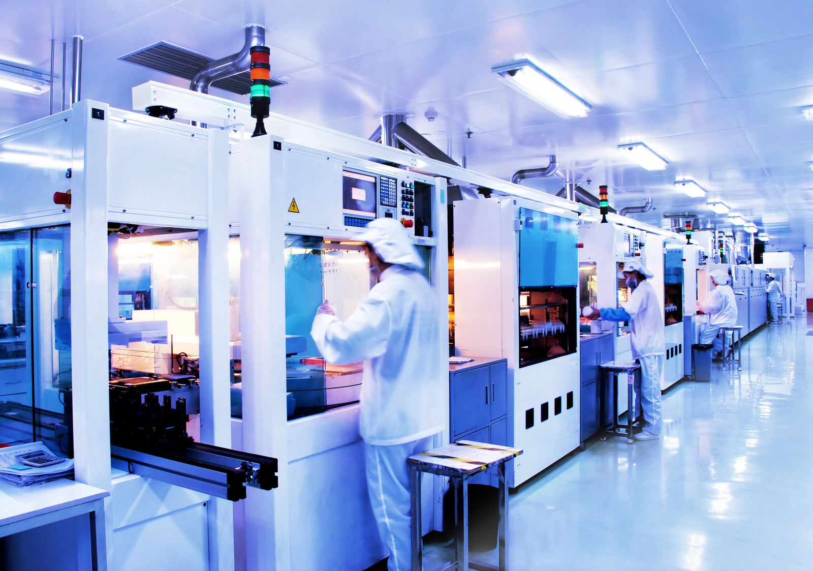
Photovoltaic Production Line          Photo Credit: canstockphoto.com/06photo

In our last post we sketched out the Solow-Swan model of economic growth that created an economic picture of per capita capital stock determining GDP, savings, and replacement investment. The addition of a simple savings model with a constant or average savings rate over a year yields the national savings, which together with replacement savings determines net savings that drives GDP growth. As a summary I list the pertinent definitions used in the model, together with their relations to other model variables. 

• GDP: The sum of values added by all producers for all goods and services, which is an aggregate representing the sum of all additions of wealth to the nation without double counting. Represented by the letter y, it is related to the number of workers l, the economy’s capital stock per worker k/l, and all secondary factors of production by a Cobb-Douglas production function of the form The factor A, called the total factor productivity, is a function of all secondary factors of production such as technology, skill-level of labor, etc. If we make the simplifying assumption that everyone works, then l is the number of the population as well as the number of workers, and y/l becomes per capita GDP and k/l, the capital-labor ratio is also the capital per capita. This is not a necessary assumption, but it does make the mathematics simpler. Let the parameter κ= k/l be the capital to labor ratio. The observed behavior of diminishing marginal productivity means that y is constantly increasing with increasing κ but increasing less and less as κ increases. For those with some knowledge of calculus, the theory requires 
• Capital: The total dollar value of the physical assets used to create wealth. It is represented with the letter k in this discussion.
• Replacement Investment: The investment required to replace worn out or obsolescent capital stock and to maintain the capital to labor ratio after population growth. The per capita replacement investment is given by  where d is the depreciation rate, the fraction of the capital stock that must be replaced due to wear and tear or obsolescence, and n is the fractional population increase rate,
• Total Investment: The total amount spent in a year for future needs rather than current consumption. This amount includes replacement investment. Total investment is presented by the letter i.
•  Net Investment: What is left over after replacement investment is taken out of total investment. If replacement investment takes all of total investment, net investment n_i = 0.
• Total National Savings: The total amount of household income and government revenues not spent on current needs, i.e. on consumption. Because the only place for savings to go is to investment, total investment must equal total savings. We then have for total investment where θ is the average savings rate for the year.

A Steady State Economy

What happens to an economy described by the Solow-Swan model depends on three functions of κ = k/l, namely the GDP per capita obtained from the Cobb-Douglas production function

the replacement investment given by

and the savings per capita given by

We will now consider the very special case where the capital-to-labor ratio κ is such that the replacement investment is exactly equal to the total savings. In that case if we were to plot the three curves versus κ, we would get something like the graph below.

For this economy the capital per capita κ₀ = k₀/l  has a value that gives a GDP value y₀ such that when it is substituted into the savings equation s₀/l = θ y₀/l, it gives a point on the savings curve that is right on top of the replacement investment curve. With the savings being exactly what is required to keep the capital to labor ratio constant, the economic system points on the three curves will not move one way or the other. There is no savings over the replacement requirements to provide for net investment, which is zero in this case. Therefore there will be no growth in the economy and κ will not increase. On the other hand there is enough savings to make all required replacement investments so that κ = κ₀ does not decrease either. The economy is truly at a steady state.

A Non-Equilibrium Economy

Next we will consider what happens when the economy starts off with a capital to labor ratio that is greater than the steady state value, i.e. we start off at κ₁ > κ₀. The situation is now as shown in the graph below.

As you can see from the graph, the amount of replacement capital required to keep the capital per capita constant is greater than the amount of savings. Not only is there not enough savings for net investment to grow the economy, there is not even enough to make all needed replacements of capital stock. As the capital stock κ decreases below κ₁ the productive capacity of the economy decreases and the system points on the three curves will follow the directions of the black arrows until they reach the steady state points at κ = κ₀. At that point there is just enough savings to make all required replacement investments and all macroeconomic changes cease, at least until something is done to change the system.

If the system had started with a κ less than κ₀, the story would be somewhat similar. In that case, however, the point on the savings curve would be above the point on the replacement investment line so that net investment could be made to increase the economy’s productive capacity, i.e. to increase the capital stock so the three system points on the three curves move toward their values at κ₀. Once they hit their steady state points, required replacement investments will have caught up to the savings curve and net investment will have shrunk to zero. The system will again be at steady state.

Lessons for Us Today

So where is the United States on the Solow-Swan Chart? First, we should note that the Solow-Swan economy we constructed was implicitly assumed to be isolated from the rest of the world; there was no foreign trade or investments.

In the real world there are such exchanges for which the United States can thank its lucky stars. Many countries, especially China and Japan, have done the U.S. the singular good favor of helping to fill the large hole of the federal government’s negative savings by buying U.S. Treasury bonds. In effect we have been able to count a portion of Chinese and Japanese national savings as ours so that we could meet all of our replacement investments and have enough left over to make at least some net investments. However, as the figure to the left shows with the yellow curve, we have had very poor economic growth over the past six and a half years. Therefore, the U.S. system points in the Solow-Swan charts above must be just to the left of the steady state points. Yet even as foreign savings have been re-routed toward the U.S. to our benefit, our own savings rate is being systematically destroyed by the present and past monetary policies of the Federal Reserve, as we discussed in the post The Importance of Personal and National Savings. More and more we need foreign purchases of our sovereign debt to help relieve the negative savings rate of the federal government and the steadily decaying savings rate of American households. Between them and the pouring of foreign savings into our economy, the average savings rate θ in our simple savings model is determined. The more  θ decreases, the closer the red savings curve in the Solow-Swan diagrams above hugs the κ axis, and the closer one gets to a situation where the savings curve intercepts the replacement investment curve virtually at the diagram’s origin. If that were to happen, decay of the economy’s ability to produce wealth would be unavoidable.

But wait! We have just mulled over what happens with a changing shape of the savings curve! All our preceding discussion of what happens to an economy has really implicitly assumed constant shapes for the three defining curves. What happens when these shapes do indeed change with time? And what changes in a society and an economy can bring about such changes in the three curves? We will address these subjects in the very next post.

GO TO HOME

Sharing is caring!