The Solow-Swan Model and Where We Are Economically (1)

They don’t pay me enough!          Photo Credit: Flickr.com/Bitterjug

OK, everyone! Put on your thinking caps because we are going to be doing some serious macroeconomics thinking. We will even be using (Oh, horrors!) some algebraic equations. The purpose for doing this will be to see what modern economic ideas can tell us about our current economic predicament.  

Before I get into the meat of this post, let me say that I got the ideas for it from an internet course I am taking on macroeconomics. I am in fact a physicist, not an economist, and I am entirely self-taught in my knowledge of economics. If you know anything about economics and have read a number of my posts, you may well have noted my stress on the more microeconomic emphasis of neoclassical economics. So I thought it would be good if I took an actual course on macroeconomics to get a more accurate view of what is going on in the Keynesian brain. In the process I have found a wondrous international consortium of universities that offer free courses on virtually any subject in existence. (You will have to pay a small fee if you want a certificate of completion.) This is such an outstanding service to humanity that I would very much like to give them some free advertising. You can find them at https://www.coursera.org. My macroeconomics course is offered by the University of Melbourne, Australia, and its professor is Dr. Nils Olekalns.

The specific economic ideas I will be using are an elegant yet simple model of economic growth called the Solow-Swan model, named after two economists who developed the model independently. At its heart is what is called a production function which relates the total economic output of a nation, or GDP, which we will represent with the letter y, to the primary input factors of capital, k, and of labor L. All of these variables are to be expressed as their values in the monetary unit of whatever country is considered. Also, we will indicate the total number of laborers with the lower case l. Also, we should note that what is considered capital is the value of all the physical stock needed to produce wealth, e.g. factories, machinery, computers, ships, etc. The most general production function can be written as

where f(k, l) is some general function of capital and labor, and A is called the total factor productivity that is a function of any and all other secondary factors of productivity, such as technology, skill-level of labor, climate, etc. The most important properties the function f(k, l) must exhibit are that it must constantly increase, but increase less and less as capital and labor independently increase. This is called the marginal diminishing productivity of those factors. The Solow-Swan model uses a particular version of the production function called the Cobb-Douglas production function, which is of the form

This expression in turn on division by the number of laborers can be expressed as

Since the function fk/l) must be an increasing function of its argument, it and the GDP y will decrease if either k decreases or the population increases, thereby increasing l. This allows us to put in the time-dependent phenomena of capital depreciation and population increase.

In any one year some fraction d of the capital stock will have to be replaced, either due to wear and tear or to obsolescence. Also, in any year the population will increase by a fraction n. For simplicity let us assume that everyone in the economy works. This is not a necessary assumption, but it makes the math simpler. Also let us define the parameter κ ≡ k/l which is the capital stock per capita. It is a trivial exercise in differential calculus to show that the change in the capital stock per capita over a single year is

where

by definition of depreciation rate d and the population increase rate n. From this we can express the decrease of the per capita capital stock in a year as

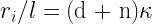
In any one year a certain amount of investment, called the replacement investment, denoted r_i , must be expended just to counteract depreciation and population increase in order to keep the per capita capital stock constant. The capital stock per capita can actually be increased only if an additional amount n_i, called the net investment, is invested. By definition, the replacement investment per capita must satisfy

 or

We now assume that there is more total investment than the replacement investment required to hold the economy unchanged. Therefore, the total investment per capita over the year includes a positive net investment and is

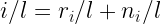
In the very last expression the net investment per capita is identified as the change in the capital stock per capita. The real lesson in all this is a country must have more investment than the replacement investment in order to get growth.

There is only one more piece to complete the model, and that is the source of investment. In order to get any economic investment at all, a portion of the nation’s yearly income, i.e. its GDP, must be held back from consumption. That portion of the GDP is the national savings. There is no source for investment other than national savings. There is household savings and government savings. Government savings is the revenues minus the expenditures, but because the government is constantly running a deficit, its savings is usually negative. This means households must save even more to make up for government’s negative savings. In principle, companies can also have savings, but after consuming for their operations and paying dividends, they often have little left to save. The Solow-Swan growth model assumes a simple savings model for the per capita savings s/l of the form

where θ is the average savings rate for the year, the fraction of GDP that is saved. Also note that the amount saved is the amount that will be invested.

We now have all the pieces of the model in hand. We will deliver all the punch lines and draw the necessary lessons for our current economic troubles in the very next post.

GO TO HOME

Sharing is caring!