The Rahn Curve, Hauser’s Law, the Laffer Curve and Flat Taxes

Hauser’s Curve                       Image Credit: Wikimedia Commons/Sugar-Baby-Love

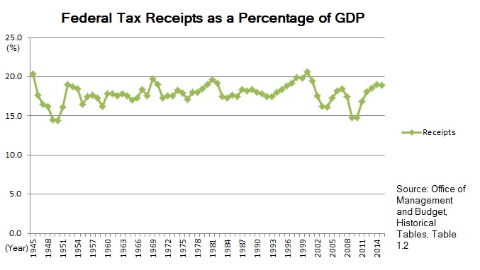
If you were to plot federal government tax revenues as a fraction of GDP versus time, you would obtain the very remarkable plot shown above. A graphical representation of what is usually referred to as Hauser’s law, it shows that despite large differences of the marginal tax rate over time, federal tax revenues have fluctuated in a very narrow band centered on a median of about 19.5% of GDP.          

The originator of this empirical law, investment analyst William Kurt Hauser, wrote in 1993, “No matter what the tax rates have been, in postwar America tax revenues have remained at about 19.5% of GDP.” The highest marginal tax rate has been as low as 28% and as high as 91% in the years 1950 through 2007. The average of tax receipts was 17.9% of GDP with a range between 14.4% to 20.9%. For tax receipts to remain within such a narrow band despite huge changes in marginal tax rates is an incredible, yet empirical fact. It can be shown that these results are specific to the United States, with its progressive income tax and lack of a national Value Added Tax (VAT). If you were to include state tax revenues and compare the resulting curve with comparable curves from the original 15 European Union countries (EU) and 34 countries of the Organization for Economic Co-operation and Development (OECD), you would get the plot shown below.

Nevertheless, even though the exact amplitudes vary between different national economies, it is striking that variations are limited to within relatively narrow bands.

This graph can be related to another theoretical curve we have already met in The Rahn Curve and the Way Out of Economic Peril. The Rahn curve gives a theoretical relationship of an economy’s growth rate as a function of government expenditures as a percent of GDP, with a shape as shown below.

If government revenues are always in a small band as a fraction of GDP, then the economy’s position is pretty much in a small segment of the horizontal expenditure axis of the Rahn curve. One other thing we learned from my post on the Rahn curve is that the U.S. economy must be on the decreasing branch of the Rahn curve. In recent years government spending must have been greater as a fraction of GDP than would have been optimal for maximum economic growth. We discovered this by making a scatter plot of the GDP growth rate versus government expenditures as a percent of GDP. Each quarter from the first quarter of 1947 to the second quarter of 2015 provides a single point on the scatter plot. The result is the plot shown below.

The data is noisy due to GDP growth fluctuating with recessions and recoveries, so it does not produce a well defined curve. However, by inspection you can see that if you fitted a straight line to this data, you would obtain a GDP growth rate that decreased with increasing government expenditures as a fraction of GDP. If you wanted to maximize GDP growth rate, you would necessarily have to reduce federal government expenditures to a smaller share of GDP.

How could we accomplish this if Hauser’s law tells us that post World War II federal government revenues were all within a few percent of 19.5 percent? As I noted earlier, there is nothing magical about the figure of 19.5%. The average government revenues of the EU and of the OECD countries had larger shares of their GDPs. If the U.S. were to make a deliberate policy of reducing expenditures to below 19.5% of GDP, expenditures would begin to match revenues, and the fact we are on the declining branch of the Rahn curve tells us that decreasing expenditures would also increase GDP growth. Smaller spending divided by a larger GDP would then give us a smaller share of GDP for expenditures.

I also noted in my post on the Rahn curve that existence of the Rahn curve also implied the existence of the Laffer curve, a plot of tax revenue versus tax rate, as shown below.

Since the federal government has almost always, within the living memory of most people, spent all of its revenue and more, we have the historical fact that if it taxes more, it will spend more. Therefore, if the economy is on the declining branch of the Rahn curve, it is also on the declining branch of the Laffer curve to the right of the revenue maximizing point. As tax rates go up and tax revenues go down, government spending as a fraction of GDP goes up and GDP growth goes down.

What this implies is the government can actually increase its revenues by simultaneously decreasing tax rates and decreasing its spending. Note that merely decreasing tax rates without also decreasing spending will not necessarily increase tax revenues. Both actions must be done to release capital assets for increasing productive capacity for larger GDP growth.

How can this be achieved? The cutting of taxes is the politically easier part (not that it would be easy), and would be easiest with the adoption of a flat tax with no exemptions, as discussed in The Ideal Tax Regime – 2. Economic growth would be especially encouraged if the U.S. switched from a world-wide tax model to a territorial model, thereby encouraging multinational corporations to repatriate overseas earnings for investment inside the United States. Also, a flat tax with no exemptions other than for low income would eliminate the wasteful habit of politicians attempting to choose economic winners and losers. Then the economic signals of free market prices, Adam Smith’s invisible hand, would direct economic assets to their optimal allocations.

How much should taxes be cut? A very big hint is given us by Hauser’s law. We know that the economy is now in a state where tax revenues are around 19.5% of GDP and that we must reduce this level. The optimal tax rate maximizing revenues must then be below 19.5% if a flat tax is used. Perhaps we should start with a flat tax of 18%, and adjust that rate as needed.

Much the harder task politically would be to actually cut government expenditures. Because of its complexity, I will discuss this part of what is needed in future posts.

GO TO HOME

Sharing is caring!