The Fed’s Labor Market Conditions Index

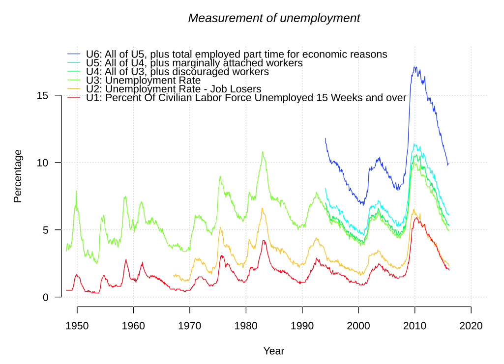
U.S. measures of unemployment          Image Credit: Wikimedia Commons/Autopilot

Wow!! The Federal Reserve so distrusted the Labor Department’s unemployment statistics that it created its own?! That is what I learned from a post by John Crudele on the New York Post website. There I read the Fed had such little confidence in Labor’s statistics that they very quietly started to compile their own measure of unemployment two years ago.   

Construction of the Labor Market Conditions Index

They called it the Labor Market Conditions Index, or LMCI. Federal Reserve documentation of the LMCI can be found in the PDF entitled Assessing the Change in Labor Market Conditions by Hess T. Chung et. al. Mathematically, it is a number formed by a relatively complex process as a composite of 19 indices that cover the following types:

1. Unemployment and underemployment indices:
   1. U3 unemployment rate
   2. Labor force participation rate
   3. Involuntary part-time employment
2. Employment indices:
   1. Private employment
   2. Government employment
   3. Temporary help services employment
3. Workweeks:
   1. Average weekly hours of production workers
   2. Average weekly hours of persons at work
4. Wages: Average hourly earnings of production workers
5. Job Vacancies: Composite help-wanted index
6. Hiring:
   1. Hiring rate
   2. Transition rate from unemployment to employment
7. Layoffs:
   1. Insured unemployment rate
   2. Job Losers unemployed less than five weeks
8. Quits:
   1. Quit rate
   2. Job leavers unemployed less than five weeks
9. Surveys of consumers’ and businesses’ perceptions:
   1. Job availability
   2. Net hiring plans
   3. Unfilled jobs openings

The mathematical details are somewhat complex, so you may wish to skip down to the next section. Each of these 19 indices are connected linearly by a dynamic factor model to a set of common factors, which are determined by a vector autoregression that eliminates noise in the data. You can find a description of dynamic factor models in the PDF Dynamic Factor Models by James H. Stock, Harvard University, and Mark W. Watson, Princeton University. Other useful internet sources on dynamic factor models can be found here and here and here.

Formally, we start with a  linear  equation of the form

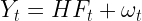
where Y_t is a column vector with 19 components, each of which is one of 19 indices composing the LMCI, and where F_t is the three-dimensional common factor vector. The 19 dimensional vector ω_t is a random noise vector. The subscript t indicates the vectors vary with time periods, The 19×3 matrix H is called the  common factor load matrix, and its components are determined by the model and the autoregression process. To get the LMCI, one must do an eigenvector decomposition of the matrix H. If θ is the eigenvector associated with  the largest eigenvalue, then the LMCI for the time period t is defined by

[Note: if you are disturbed by the idea non-square matrices can have eigenvectors and eigenvalues, as I was, look at the Mathematics Stack Exchange posts here and here. It turns out you can find approximate eigenvectors and eigenvalues using Singular Value Decomposition (SVD).]

Advantages of Using the LMCI

The Federal Reserve calculated the LMCI monthly from the beginning of 1976 to November 2014 to obtain the plot shown below.

Note that the periods of greatest change of the LMCI are during periods of recession and subsequent recovery. If instead of plotting the LMCI, one plotted the average monthly change in the LMCI, the following plot would be obtained.

Now the peaks are on the periods of maximum growth and the troughs are centered on the periods of recession. This is enough to certify the LCMI as a coincident economic indicator.

Use of the LCMI as a coincident indicator indicating labor market conditions is only part of its advantage. A second big advantage is that it gives estimates of each of the 19 indicator components making up the index with past noise filtered out, as components of the vector

In particular, one component of that vector is the prediction for the U3 unemployment rate.

Current Labor Market Conditions

John Crudele reported in his post the current U3 unemployment rate predicted by the most recent calculation of the LCMI in February is 5.8%. That is a heck of a lot higher than the 4.9% official jobless rate given out by the Labor Department. Crudele notes that it also explains why Janet Yellen and company on the Federal Open Market Committee (FOMC) are so reluctant to raise interest rates while supposedly the economy has reduced unemployment to below their target rate of around 5.0%. The FOMC has been reluctant to actually state what target they were pursuing, but since U3 unemployment was 5.0% in December when they raised the Fed funds rate, presumably 5.0% is in the neighborhood of their target.

This large difference of almost a full percentage point between the LCMI derived rate and the Labor Department rate brings up the question of just how accurately the unemployment rate could be determined. We can not depend just on the number of claims for unemployment insurance, as that would leave out all the unemployed who have run out of benefits, and some delay applying, and there are some who never apply. Instead, the U.S. Census Bureau takes a monthly survey called the Current Population Survey (CPS), presently over about 60,000 eligible households with around 110,000 individuals. Among the questions asked are ones about labor force activities that include whether or not people are holding or seeking jobs. According to the Bureau of Labor Statistics

…the survey responses are “weighted,” or adjusted to independent population estimates from the Census Bureau. The weighting takes into account the age, sex, race, Hispanic ethnicity, and state of residence of the person, so that these characteristics are reflected in the proper proportions in the final estimates.

A sample is not a total count, and the survey may not produce the same results that would be obtained from interviewing the entire population. But the chances are 90 out of 100 that the monthly estimate of unemployment from the sample is within about 300,000 of the figure obtainable from a total census. Relative to total unemployment—which ranged between about 7 and 15 million over the past decade—the possible error resulting from sampling is not large enough to distort the total unemployment picture.

However, one should not take the Bureau at its word about the results not containing large systematic errors. The difference between the Fed’s LMCI result and the Labor department’s should teach us that. One important possible source of error is the seasonal adjustments applied to the unemployment rate. Change the model for seasonal adjustment and the government has some latitude to do some convenient fibbing. Leeway for fibbing can also be given by adjusting methods for eliminating noise in the data. In addition, there are all those adjustments for “age, sex, race, Hispanic ethnicity, and state of residence of the person!”

Caveat emptor!

Views: 2,258

GO TO HOME

Sharing is caring!