How New Keynesians Explain 1970s Stagflation

Dr. Jimmy Carter’s Stagflation Advice: “I’m Going To Give It To You Straight—I Don’t Have Any Idea What I’m Doing.”                              Image Credit: Flickr.com/cliff1066

We are just about at the point where we can understand the New Keynesian explanation for the stagflation of the latter half of the 1970s.  First, however, we need to look at the New Keynesian view of inflation shocks. What we saw earlier in the post New Keynesian Adjustments for Inflation was how the New Keynesians used ideas about short and long run equilibrium under inflation’s influence to explain a  positive demand shock. New Keynesian ideas can look at several different kinds of “shocks” to the economy that can drive an economy away from a general equilibrium of both short and long run equilibrium, and at how under the influence of purely market forces, the economy will self-correct and return to a new general equilibrium, sometimes at the cost of a higher interest rate. Besides the positive demand shock we have already examined, there is a negative demand shock, and positive and negative supply shocks that can also be called positive and negative inflation shocks. Why are supply shocks and inflation shocks identical? This is because in a short run equilibrium, short run aggregate supply is completely determined by the inflation rate in the New Keynesian model.

So our first item of business is to look at a positive inflation shock, that is the inflation rate increases. If the inflation were to decrease, we would be looking at a deflation shock. We postulate that just before an unexpected jump in inflation, the economy is at the point (y*, π₀) on both the Long Run Aggregate Supply (LRAS) line, and the Short Run Aggregate Supply line SRAS₀ [Also known as the Inflation Adjustment line (IA₀)], as shown in the figure below.

Therefore we start with the system in a state of general equilibrium. We then postulate that for whatever reason, economic events create a sudden, unexpected increase in inflation from π₀ to π₁. It is important to note the implicit assumption that whatever created the  inflation did not shift the Aggregate Demand line AD₀, nor the LRAS line, but did shift the IA₀ line to IA₁. This is why the shock is called an inflation shock. If both the AD and IA lines were shifted, the system would be suffering both a demand shock and an inflation shock simultaneously.

So how does an economy adjust to such a positive inflation shock? First of all, as the short run aggregate supply line shifts from IA₀ to IA₁, the amount demanded by consumers transitions along the AD₀ line from (y*, π₀), to (y₁, π₁), as indicated by the black arrow in the figure above. As the inflation increases, households and companies will buy less to stay within their means. When the economy reaches the intersection between AD₀ and IA₁, it enters a short run equilibrium and momentarily stops. However in the process it has opened a contractionary output gap, ( y₁ – y* )/ y*. Because, households and companies have reduced their expenditures, the supplying companies begin to lose profits. They can not increase their profits by increasing prices (i.e. by increasing the inflation rate), so they will seek to increase their sales volume by reducing their prices in a way that maintains their profits, which are equal to the product of sales volume and price. By reducing prices, the companies cause the inflation rate to decline, and the economy retraces its steps along the AD₀ line from IA₁ to IA₀, as indicated by the dotted black arrow above. It ends up finally in its original state of general equilibrium at (π₀, y*). What is extremely important for all of this analysis is the New Keynesian assumption that inflation will always adjust automatically through market forces to output gaps.

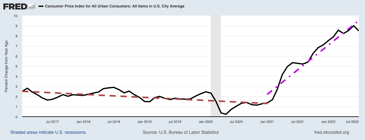
There is positive evidence that economies behave in this way from U.S. CPI data measuring the inflation rate, as can be seen in the Federal Reserve Economic Database (FRED) graph below. If the inflation rate increases rapidly before a recession, one can see the inflation decrease monotonically until the end of the recession. You can also see that in recent decades that inflation tends to return to a long run average of around 2.5%, demonstrating inflation inertia.

This is a very important case for our purposes, because it is about half of what New Keynesians believe caused the great stagflation of the 1970s. During the 1970s the dominant economic philosophy was not that of the New Keynesians, but that of the neo-Keynesians, who adhered to to the original neoclassical synthesis . They did not have the New Keynesian models we have been developing in this and the previous two posts. Instead, they used the original, simple version of the Phillip’s curve to include inflation in their models, and in that framework there was no way that a contractionary output gap could coexist with increasing inflation, as was the case with stagflation, but should lead to decreasing inflation. In New Keynesian language, what the neo-Keynesians thought was happening was a positive inflation shock as illustrated below. The inflation or supply shock was introduced by a worldwide shortage of oil due to political events and the lessening of output from Western oil fields (see 1973 oil crisis and 1979 energy crisis).

The 1970s neo-Keynesians knew that if the situation were as they thought (which it was not), then the economy under market forces would retrace its steps back to the original general equilibrium at (y*, π₀). Nevertheless, the neo-Keynesians thought that allowing natural market forces to take the system back to general equilibrium would take a very, very long time, maybe as long as three years or more. Considering this result to be unacceptable, they decided to “stimulate” the economy by decreasing interest rates to increase aggregate demand and shift the AD₀ curve to AD₁. Then the economy could be allowed to move under market forces along IA₁ from point B to what they thought was the general equilibrium at point C with coordinates (y*, π₁) as in the figure below. The “only” cost would be the inflation level would be permanently increased from π₀ to π₁.

But they had been fooled! Instead what had happened was the events had been so damaging that the potential GDP itself had decreased from y* to y**, with the long run aggregate supply moving from LRAS₀ to LRAS₁ as shown below. What the neo-Keynesians at the time thought was a short run equilibrium with a contractionary output gap was actually a new general equilibrium! When they pushed the aggregate demand curve from AD₀ to AD₁ and the economy moved from point B to point C along IA₁, they were actually opening an expansionary output gap rather than eliminating it. Then under the influence of the expansionary output gap, more inflation was generated and the economy moved along the aggregate demand curve AD₁ to another general equilibrium at point D at an even higher inflation rate of π₂.

At each time the Federal Reserve attempted this, they always returned to a general equilibrium at a GDP of y** at a higher inflation rate. At the time everyone believed that inflation was accelerating while economic output was stagnating. This is the New Keynesian explanation for stagflation during the 1970s.

Of course, the monetarists among them, Milton Friedman chief among them, had a slightly different interpretation. They thought that the Phillips curve allowed increases in GDP at the expense of higher inflation only up to the time inflationary expectations were deeply ingrained among people. They would then demand “inflation adjustments” to their wage increases that generated further inflation. Eventually the runaway inflation became so large that the increase in inflation could no longer be passed on to consumers by price increases. Stagflation then resulted. One could easily argue that both points of view are highly compatible, After all, New Keynesian economic doctrine evolved from this experience partially as a reaction to Friedman’s monetarist critique.

I believe you now have what you need to get an appreciation for what New Keynesian economic theory is all about. In the  very next post, I will give you what I think is very, very wrong with it, and in fact very wrong with every brand of Keynesian thought.

GO TO HOME

Sharing is caring!