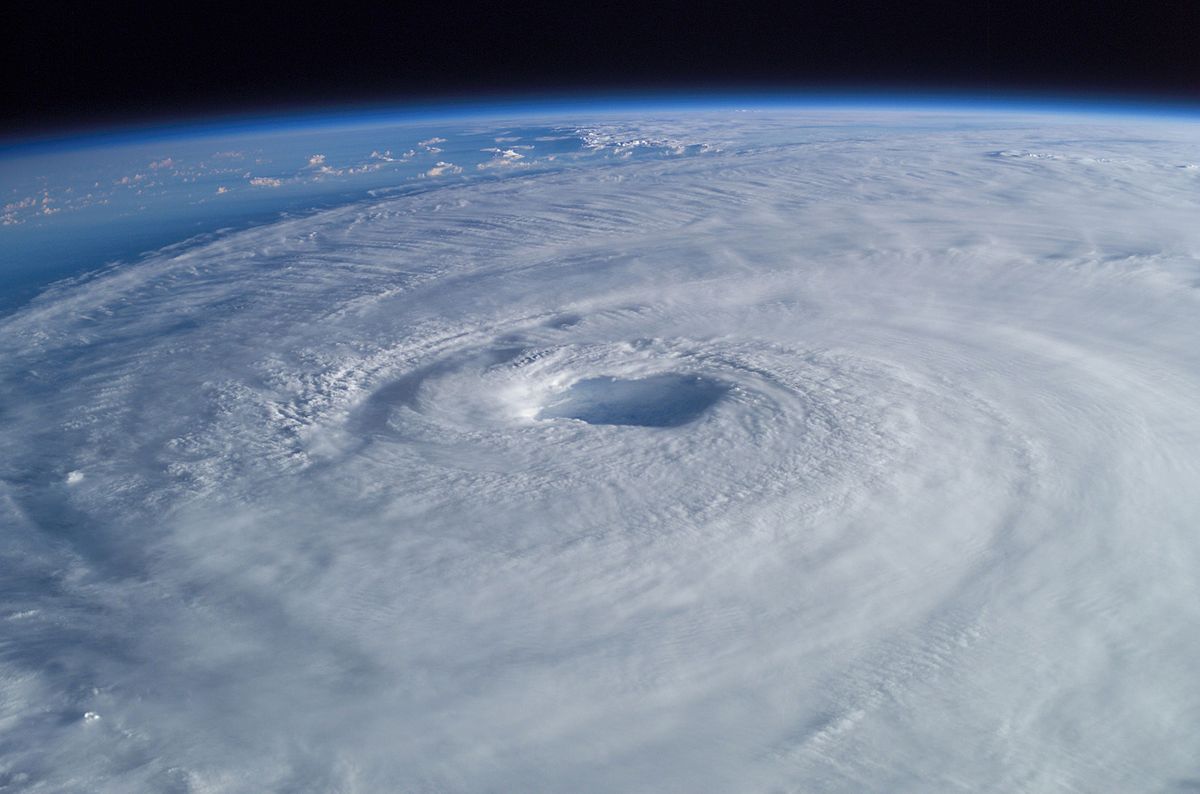
Hurricane Isabel, a category 5 hurricane, seen from the International Space Station in  September 2003. This deadly storm had many of the same system characteristics in the planet’s weather that a government Keynesian “stimulus” program has on an economy.
Photo Credits: Wikimedia Commons/Image Courtesy of Mike Trenchard, Earth Sciences & Image Analysis Laboratory , Johnson Space Center.

Organized. Deadly. Destructive. Those were major qualitative characteristics of Hurricane Isabel in September 2003, and they are much like some of the qualitative characteristics of a government’s Keynesian “stimulus” program in an economy. In fact, the analogy goes far deeper than mere metaphor, as they are closely related mathematically in their descriptions inside their respective systems: in the planet’s weather system in the one case, and in a country’s economy in the second.

Two Systems: Weather and Economic

To describe any system, a person must discover the variables that completely describes the system’s state at any one time and list their values. To go further and predict how the system will evolve into a future state, we must know each variable’s “equation of motion”. As you will soon see, both weather systems and the economic systems of individual countries and of the world have largely defeated the human intellect to date. But first we must look at how systems in general are described.

Let us begin with weather systems. A weather system is made up of countless molecules of different species that compose the atmosphere. Boundary conditions are imposed on it by the surface of the Earth and the more diffuse boundary layer with the vacuum of space. The energy driving its behavior comes almost entirely from incident radiation from the sun, although the force of Earth’s gravity has a big influence with its partial transformation into a Coriolis force with the Earth’s rotation, and with its chain on molecules resisting their loss to the vacuum of space. To completely describe the various motions of the atmosphere at a particular time, you would have to define six quantities for every molecule and particulate in the atmosphere: the three coordinates of its position and the three coordinates of its momentum. If the number of particles of all species in the atmosphere is N (a truly humongous number!), the total number of quantities defining the state of the system is 6N.

In addition the inhomogeneous existence of clouds greatly affects Earth’s weather since it affects how much of the Sun’s incident radiation reaches the inner atmosphere, the troposphere, to be absorbed and affect the troposphere’s temperature. I describe this phenomenon in my post theme of global warming. No computer simulation encompassing the entire Earth’s atmosphere of which I am aware adequately treats the effects of clouds. And of those models, absolutely none handles the variation of cloud cover caused by cosmic ray intensities in the lower atmosphere, which in turn are controlled by the intensity of the solar wind  around the Earth.

In principle, you should be able to solve Newton’s second law of motion to describe the future state of motion, but a number of practical considerations stand in our way. To begin with, no computer has yet been built nor probably will be built for a very long period of time that can store that number of variables in memory, nor compute the results from Newton’s second law in a reasonably finite amount of time (say, within the lifetime of the youngest baby on Earth). This means we have to greatly simplify the description to have any hope of a solution.

As it turns out, this task can be performed by considering the different species of particles  as composing different species of fluids. Each fluid is described as a continuous field (a field is just a variable that has a different value at every position and time) giving the density of particles at every position in space. Now the computational complexity of the problem is reduced from the 6N coordinates of each particle to a smaller number of fluid densities at grid points gridding the space occupied by the atmosphere, times the number of species of atmospheric particles. This still gives a very large number of variables to store in memory and calculate, unless you make the grid point density very coarse indeed.

One of the first people to approach the computer solution of this problem was the American mathematician and meteorologist, Edward Lorenz, at the Massachusetts Institute of Technology. He was the man who coined the term “Butterfly Effect”, popularized by the motion picture Jurassic Park.

Clip from the 1993 movie Jurassic Park describing the Butterfly Effect

What Lorenz discovered in his computer simulations was the incredible sensitivity of the weather system to initial conditions. Mere roundoff errors in the initial  conditions of computer variables were enough to make computer simulations not reproducible. In a 1963 paper “Deterministic Nonperiodic Flow” in the Journal of the Atmospheric Sciences, he wrote:

Two states differing by imperceptible amounts may eventually evolve into two considerably different states … If, then, there is any error whatever in observing the present state—and in any real system such errors seem inevitable—an acceptable prediction of an instantaneous state in the distant future may well be impossible….In view of the inevitable inaccuracy and incompleteness of weather observations, precise very-long-range forecasting would seem to be nonexistent.

Small round-off errors in the inputs of initial conditions would be sufficient to produce huge differences in the system state at a later time. The coining of the term “butterfly effect” came from the title of one of his papers in 1972, “Predictability: Does the Flap of a Butterfly’s Wings in Brazil Set off a Tornado in Texas?”. This started the study of chaotic systems as systems sensitive to very, very small changes in initial conditions. We will discuss the chaos of weather systems, and indeed of economic systems (aka economies), a bit more in the next section on Chaotic Systems, but first we need to explore how weather systems and economic systems are so very similar.

We described a weather system in terms  of a collection of variables giving both the position and momentum for every molecule in the system. We then simplified the problem by many orders of magnitude by aggregating particles into fluids. The coordinates describing the state of the system have now become the density and fluid velocity for each species of molecule on a 3-dimensional grid. Also, to take account of random variations of particle velocity around the local fluid velocity, we must introduce a temperature field.  A temperature is a measure of the amplitude of random velocity fluctuations around the fluid velocity; or equivalently it is a measure of the kinetic energy in the random motions of the molecules. Remember, we must make the spatial grid on which we define these variables as coarse as we can possibly make it without sacrificing important spatial variations. A very difficult task, indeed!

We can do something very similar to describe the state of an economic system. The interactions between molecules in a weather system are almost entirely collisions between pairs of molecules, when two molecules come very close to each other. We say that the interactions are local in the state-space describing the system’s state, which is given by the positions and velocities of all the particles. If we were to think of economic systems in the manner of physicists thinking about a weather system, we would first define the basic interactions in an economic system and discover the state-variables that are changed by those interactions.

In any economic system, whether it be socialist or capitalist, the basic economic interactions are between pairs of suppliers and consumers who make deals to exchange goods for money. These basic interactions occur for every good in the market. The analogue for Newton’s first law of motion (a particle’s momentum does not change unless a force acts on it) is the law of supply and demand (the supply and demand for a good are determined by its market price, which does not change unless the availability of the good changes), and the analogue for Newton’s second law (a change of a particle’s motion is determined by a force acting on it) is the law of marginal utility (changes in supply and demand of a good are determined by changes in the good’s availability, or by changes in consumers’ desires for the good).  The state space for an economy could be defined from the number of suppliers and consumers (demanders) at every possible pair of price and quantity of goods exchanged, We must specify this for every good in the marketplace. The densities of suppliers and demanders for every possible exchange will be determined by the price and quantity of every proposed deal. That is, the state space is the price and quantity for every good in the economy, and the density of suppliers in that state space is the supply curve in the law of supply and demand, while the density of demanders is given by the demand curve.

Just as with a weather system, all interactions in an economic system are local between individual pairs of suppliers and demanders. That is, economic transactions, i.e. interactions, can occur only if a supplier and a demander can agree on a quantity and price for the exchange. In yet other words, the supplier and demander are at the same position in the state space of supply and demand when they interact.  In both weather systems and economic systems, the interactions between the basic components of the system are local in their respective state spaces, and they both have a huge number of degrees of freedom, which are the coordinates of the interacting components in the state-space. As it turns out, these shared qualities of economies and weather systems also make them both chaotic systems.

Chaotic Systems

What differentiates a chaotic system from a non-chaotic system is the extreme sensitivity of a chaotic system to its initial conditions. What this means is the following: Suppose you prepare two otherwise identical systems, but you differ their system states infinitesimally at the time (call it t=0) you release them to evolve. Scientists have done this sort of thing countless times in both experiments and computer simulations. If your two almost identically prepared systems are chaotic, you will witness a very dramatic difference in their behaviors after a short period of time.

What causes a weather system to be be chaotic? One obvious reason is the huge number of particles that can interact, i.e. the number of the state variables of particle position and particle velocity that can be changed randomly by random collisions between particles. The second, not-so-obvious reason is the interactions between particles are local in the state space. Their interaction is not strong, i.e. the transfer of momentum is not large, unless the two interacting molecules are very close to each other in both position and velocity. They must be very close to each other in position because of the limited range of the interaction force. However, they must also be very close in velocity or momentum. Otherwise, the particles will zip by each other, providing a very limited time over which momentum can be exchanged via the limited-range of the interaction force.

Now visualize what happens to two otherwise identical weather systems defined in two runs of the same computer program simulation when their initial conditions are very subtly different. Suppose in both simulations we define two fluid flows, two winds, that collide with each other.

What happens to the two flows depends on how much energy they have in their respective fluid velocities. If one is much stronger with greater energy and momentum, it will disrupt the other flow more through random collisions of its molecules, than the other flow will disrupt it. The weaker flow will then be disrupted into smaller whirls, which will then be disrupted into even smaller eddies until all trace of organized, directed fluid motion has disappeared into eddies of different sizes. Even the stronger wind would be somewhat disrupted in this way, although to a lesser extent.

Even if there were just one wind in the initial condition, collisions with a motionless background fluid would eventually disrupt the fluid flow into turbulent eddies. The exact details of where and when the eddies appear, and the directions in which whole eddies travel will depend on an average over a large number of molecules. Multiple collisions will have occurred before the flows begin to separate into eddies, and the exact details of the eddy creations will depend on the initial particle positions and velocities in the organized initial wind or winds. For example, the directions of the fluid velocities of the winds in our two simulations might be subtly different because of the small differences in the initial conditions of the two computer runs. The winds in the two simulations will then travel to two, perhaps very different spatial positions when they begin to fall apart. It is in this way that a system of fluids like a weather system becomes very dependent on initial conditions, and why it is a chaotic system.

Why is it important for the interactions between system components to be local in the state space? It is only in that way that the system is dominated by collisions between the components, and that any fluid disturbance would travel for some distance before it decayed into eddies. If the range of the interaction were infinite and a particular molecule interacted with all other particles at the same time, the other molecules would quickly drag a molecule in the wind to a stationary state due to their collective inertia.

Everything I have just written about a weather system could be repeated for an economic system, as the reasoning depends sensitively on two postulates. The first is coordinates of system components provide a large number of degrees of freedom. This assumption implies that interacting system components (suppliers and demanders in an economic system) can move fluidly in the system state space. If they could not, then the number of degrees of freedom would be reduced. A completely non-fluid system, a solid, can be made up of many millions of particles, but has only six independent degrees of freedom: the three coordinates of the center-of-mass, and the three components of its center-of-mass velocity. The other degrees of freedom of the coordinates and velocities of the constituent particles have been eliminated by the constraining forces holding them in a lattice to form the solid. The only way for the degrees of freedom to be a large number is if the particle motions in the state space are fluid.

The second postulate is that the system component interactions are local, i.e. the interacting components are very close to each other in state space. This is needed to ensure the system remains fluid and that the interactions are collisions that help randomize component motion in the state space. In an economy, such motion would be interpreted as a supplier moving from one consumer to another, and vice versa. Even physical concepts like inertia (“sticky” prices and wages, borrowing an idea from the New Keynesians), distance (involving number of trades of intermediate goods to the final good, and differences between suppliers and demanders of prices and quantities), and momentum(prices times quantities) can be introduced.

Does this mean that a chaotic system can never be stable? Not at all! If sources of disturbances remain small and either constant or decaying and the entire system is allowed to self-adjust, a quasi-static equilibrium, i.e. an equilibrium that changes slowly, can form. You can see this happening when you get a week of relatively constant good weather. As long as the boundaries of the relatively constant good weather are not crossed by disturbances such as cold fronts or warm fronts, the good weather will remain stable.

In an economy,  consider an economic sub-space that contains a company, its suppliers, and its customers, and the internal boundary that encloses that sub-space. If economic disturbances do not cross that internal boundary, the combined laws of supply and demand and of marginal utility (also known as “Adam Smith’s Invisible Hand”) will guide that sub-system to a local equilibrium. What a local equilibrium means in the context of an economy is that the density of suppliers and demanders of a good in its region of the economy’s price-quantity state space remain relatively constant.

However, if really large disturbances (often called supply or demand shocks in more conventional pictures of the economy) cross the local boundaries surrounding an industry, the number of suppliers willing to supply a customer with a good at a quantity and price on which both can agree might drastically fall or even vanish altogether.  This is what we must discuss next.

Globally Perturbing a Chaotic System

If a chaotic system is globally perturbed, it’s perturbed state almost by definition will be unstable. In an economy it would upset supply and demand balances over much if not all of the economy, such that either expensive surpluses or damaging shortages are created according to the law of supply and demand. The oil supply shocks  of 1973-1974 and of 1979 were large perturbations of this nature, which in both cases generated recessions. Before we discuss large perturbations of this nature  and their sources in economies, let us look at the dramatic and deadly perturbation of a hurricane in the weather system.

An instability, either in the economy or in physical phenomena, can grow only while there is some fuel available to feed its growth. Once that instability consumes all the available fuel, it ceases to exist and the perturbation decays to nothingness. This is dramatically the case with hurricanes (aka tropical cyclones). They typically are born over the warm water of tropical oceans near the equator. In the beginning warm, moist air with evaporated water from the ocean’s surface rises over cooler atmospheric air above the oceans. Because the rising warm, moist air rises, it leaves a volume below it with less air and lower air pressure. Cooler air surrounding the disturbance swirls into the lower air pressure volume, causing the rising air to rotate in the opposite direction to conserve angular momentum. When it is heated by contact with the warm water surface, the descending air absorbs evaporated moisture and rises as well. As the hurricane rotates increasingly faster, a funnel or eye of the hurricane is formed and becomes well defined. This sets up a structure as shown below.

Hurricane formation generally peaks in late summer when the difference between warm sea temperature and cooler atmospheric temperature is at its greatest. As long as the sea temperature is warmer than the cooler air above the cirrus shield over the hurricane’s eye, the hurricane will continue to grow in strength with the wind speed of the rotating storm increasing. As the storm moves across the sea’s surface, the relatively quiescent air of the atmosphere surrounding the hurricane will collide with it. The molecules of the quiescent air are then set in rotation by colliding with hurricane molecules and become part of the storm. In those collisions the formerly slow atmospheric molecules will absorb a small fraction of the momentum of the storm molecules, which is readily resupplied by more moist air sucked up the wall of the eye. Below is an amazing video taken from an orbiting satellite of the formation of hurricane Katrina in 2005.

Whenever a hurricane makes landfall or travels over colder water, the storm loses its fuel and the frictional forces from the surrounding (relatively) quiescent atmosphere causes the storm to break up onto successively smaller eddies until the storm no longer exists.

This rendition of the birth and death of hurricanes has two important lessons for us in the context of chaotic systems.

1. Large, well structured perturbations in an otherwise chaotic system can be generated by the provision of some kind of fuel that drives an instability. The source of this fuel can often be found in the boundary conditions of the system. In the case of hurricanes, the source for this fuel is a warm ocean water boundary heating water-saturated air that rises.
2. Whenever a large-scale perturbation travels over a boundary that cuts the perturbation off from its fuel, the perturbation ceases to grow and the components making up the system (air molecules in the case of the weather system, and suppliers and consumers in the case of an economy) will interact to destroy the large scale perturbation.

In the case of an economy, the fuel for large scale perturbations is often the lack of something essential  for economic activity rather than the provision of something. This is because an economy is a social system driven as much by human psychology  as by the physical availability of resources. If people are denied economic resources they desperately want or need for their functioning in society, they will do all that they can to minimize their wants. This is the case for supply shocks where needed resources, such as oil, are suddenly in short supply.

We can also be denied what we need in the wide-spread perturbations created by foolish government actions attempting to stimulate the economy. By allocating a large fraction of the economy’s economic resources, the government denies those resources to private applications that do more to satisfy the actual wants of people. In some cases government allocation of resources are absolutely necessary for the survival and well-functioning  of society, as in defending us from ISIS or deterring the military threats of Russia, China, and Iran, However, for the past half century or so progressive politicians in the federal government have systematically plundered Social Security of its assets, leaving un-marketable special issue Treasury bonds, essentially federal IOUs, in their place.  In this way they could get their hands on Social Security funds to spend on their favorite federal government programs. Now that Social Security is expending more than it receives in payroll taxes, the government must pay for the gap. This plus the expenditures on the other two big entitlement programs, Medicare and Medicaid, now swallow up approximately two-thirds of the federal budget, and it is also the fastest growing part of the budget.

Having created such a large systematic and global perturbation on the economy, the government has placed itself in an untenable and unsustainable economic position. The growth of government expenditures is now mostly in the two-thirds of the budget that is entitlement spending. The Heritage Foundation has estimated that by 2035, less than two decades from now, if nothing is changed in federal expenditures, then entitlements (Social Security, Medicare, and Medicaid) will absorb around 34 percent of the GDP. Not of the federal budget, but of the GDP!  However, the empirical Hauser’s law limits government tax revenues to around 19% of GDP. Unless the federal government finds some way to “repeal” Hauser’s law, they will not be able to fund even the requirements for the entitlements. Sometime between now and the end of the 2020s, entitlements plus paying the interest on the national debt will soak up every single penny of federal revenues. Then the government will not be able to pay for our defense against ISIS, Russia, China, or Iran. Then the Government will not be able to pay for enforcement to ensure  people pay their taxes.  What poetic justice!

Yet, let us suppose the government finds some way to “repeal” Hauser’s law and can wrest more than 19% of GDP away from its citizenry in taxes. Every x% of GDP it yanks from the private sector economy and uses to fund its own financial needs is x% that will not be available for U.S. total investments. How long before total investments are less than replacement investments and we find ourselves in permanent depression? How long before Atlas Shrugs?

Now for the good news.

It will not be long before the federal government will be entirely incapable to enforce  its demands, because it will lack the resources to do so. At that point the decisions on how to allocate the capital resources of the nation will revert to the private sector. Seeking profits, each company will allocate resources to maximize its profits, which means producing to meet needs for which the people are willing to pay. Gradually, the chaotic economy will heal itself from the distortions created by the federal government, as it seeks local supply-demand balances required by a chaotic economy.

Life in such a scenario would be very, very difficult, since all social safety-nets maintained by the federal government would follow that government into financial destruction. In addition, all law enforcement would revert to local and state law enforcement, at least for those states capable of not following the national government into financial oblivion..

What worries me the most about such a scenario is the national defense, since in that scenario there would be no U.S. Army, Navy, or Air Force, because the federal government would no longer exist financially. How will we fend off ISIS, Russia, China, and Iran? What gives me hope is that those nations are in even tougher financial shape than we are and may be totally absorbed with their own problems to care much about conquering a foundering United States.

Yet, if we can avoid being conquered after the U.S. government collapses financially, the reversion of control of the economy to the private sector should at least ensure healing of the economy. At some point we should be capable of building a new national government — should we care to do so.

What This Should Teach Us

If we are wise, what this should teach us is to be very reluctant to allow government to monkey around with the inner mechanisms of the economy. If we can halt the slide of the economy into federal government control and allow the economy to heal itself, and if we can actually cut government expenditures, then we might have some chance of avoiding the financial collapse of the federal government. Maybe.

Views: 3,511

GO TO HOME

Sharing is caring!